Welcome
Welcome to MesoHOPS! Here, we will discuss the basics of how to initialize and run a mesoHOPS object. Make sure to check out our codebase on github! Now, let’s get started. The code is divided into six main classes. We’ll take you through the structure and function of each, and then provide an annotated example of running a trajectory with the module.
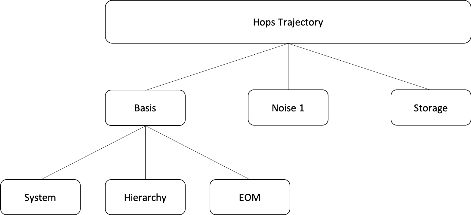
Hops Trajectory
HopsTrajectory is the class that a user should interface with to run a single trajectory calculation. To initialize a HopsTrajectory object, several parameters are needed. We split the parameters into a number of dictionaries:
System Parameters
Hierarchy Parameters
EOM Parameters
Noise Parameters
Intergration Parameters (these are not involved in any of the objects below, but are put directly into HopsTrajectory)
Each dictionary of parameters is detailed further in the documentation of the subclasses listed in the Hops System section below. Once an instance of the HopsTrajectory class is created there are three methods that the user will want to call:
make_adaptive(delta_h, delta_s)
initialize(psi_0)
propagate(t_advance, tau)
Make_adaptive() transforms a not-yet-initialized HOPS trajectory from a standard HOPS to an adaptive HOPS approach. The inputs delta_h and delta_s define the bound on the derivative error allowed for the hierarchy and state basis. The initialize() method initializes the trajectory module (whether adaptive or not) by ensuring that each sub-component is prepared for propagating a trajectory. The input psi_0 is the wave function at the initial time. Finally, propagate() performs integration along fixed time-points to propagate the wave vector. The inputs t_advance and tau correspond to the total length of the time axis of the calculation and the time step of integration, respectively.
Hops Basis
HopsBasis is a class that forms the basis set for a HopsTrajectory. HopsBasis contains three other classes that mediate the interaction between HopsTrajectory and HopsBasis: HopsSystem, HopsEOM, and HopsHierarchy. Every HOPS calculation is defined by these three classes.
Hops System
HopsSystem is a class that stores the basic information about the system and system-bath coupling. The parameters needed for HopsSystem are:
Hamiltonian - A Hamiltonian that defines the system’s time evolution in isolation
GW_sysbath - A list of parameters (g,w) that define the exponential decomposition of the correlation function
L_HIER - A list of system-bath coupling operators in the same order as GW_SYSBATH
L_NOISE – A list of system-bath coupling operators in the same order as PARAM_NOISE1
ALPHA_NOISE1 - A function that calculates the correlation function given a user-inputted function
PARAM_NOISE1 - A list of parameters defining the decomposition of Noise1
Hops Hierarchy
HopsHierarchy defines the representation of the hierarchy in the HOPS calculation. The parameters needed for HopsHierarchy are:
MAXHIER - The maximum depth in the hierarchy that will be kept in the calculation (must be a positive integer)
TERMINATOR - The name of the terminator condition to be used (or False if there is none. Currently, no terminators are implemented)
STATIC_FILTER - Name of filter to be used (‘Triangular’, ‘LongEdge’, or ‘Markovian’)
Hops EOM
HopsEOM is the class that defines the equation of motion for time-evolving the HOPS trajectory. Its primary responsibility is to define the derivative of the system state. The parameters for HopsEOM are:
TIME_DEPENDENCE – Boolean that selects whether system Hamiltonian is time-dependent
EQUATION_OF_MOTION – Name of EOM to be used (currently, only ‘LINEAR’ and ‘NORMALIZED NONLINEAR’ are supported)
ADAPTIVE_H – Boolean that selects whether the hierarchy should be adaptive
ADPATIVE_S - Boolean that selects whether the system should be adaptive
DELTA_H - The delta value (derivative error bound) for the hierarchy
DELTA_S - The delta value (derivative error bound) for the system
Hops Noise
HopsNoise is the class that controls a noise trajectory used in a calculation. The parameters for HopsNoise are :
SEED - An integer-valued seed for random noise or None, which will generate its own random seed that the user will not have access to
MODEL - The name of the noise model to be used (‘FFT_FILTER’, ‘ZERO’)
TLEN - The length of the time axis (units: fs)
TAU - The smallest timestep used for direct noise calculations (units: fs)
Hops Storage
HopsStorage is a class that is responsible for storing data for a single instance of a HopsTrajectory object. HopsStorage has no inputs. HopsStorage can store the following data
The full wave function
The true wave function
The memory terms
The time axis
The current hierarchy elements
The amount of auxiliary members being used in the hierarchy basis
The amount of states being used in the state basis
Adaptivity
The main draw of this software is the adaptive HOPS (adHOPS) approach. This allows us to take advantage of the locality of mesoscale open quantum systems and greatly reduce computational expense. For an in-depth look at adHOPS, please refer to [Varvelo et al.]. The derivative error bound (delta) controls the ‘amount of adaptivity in a trajectory’ with a delta value of 0 being a full HOPS trajectory. We have two delta values in MesoHOPS, DELTA_H and DELTA_S, representing the value of the adaptivity in the hierarchy basis and value of adaptivity in the state basis, respectively. Depending on the use case a user may decide to only make a single basis adaptive and leave the other basis empty (e.g., only setting the DELTA_H value) or to make both basis adaptive. The most important thing for the user to understand is that with decreasing delta the results are more accurate, but the computational cost increases. When using equal values for DELTA_H and DELTA_S, we will usually refer to the square root of the sum of these terms squared simply as “delta.”
Running a Trajectory
To run a trajectory, these should take the following steps:
Initialize an instance of HopsTrajectory using the parameters outlined for HopsTrajectory
Leave it as a HOPS trajectory or change to an adHOPS trajectory using make_adaptive()
Initialize the trajectory using initialize()
Decide on the time axis and time step of integration and run the trajectory using propagate()
Sample Trajectory
# We will be simulating a linear chain of pigments, with each pigment approximated as a two-level
# system. The chain is 4 pigments long, and the excitation begins on the 3rd pigment.

# Import statements
import os
import numpy as np
import scipy as sp
from scipy import sparse
from mesohops.dynamics.hops_trajectory import HopsTrajectory as HOPS
from mesohops.dynamics.eom_hops_ksuper import _permute_aux_by_matrix
from mesohops.dynamics.bath_corr_functions import bcf_exp, bcf_convert_sdl_to_exp

# Noise parameters
noise_param = {

    "SEED": 0,  # This sets the seed for the noise
    "MODEL": "FFT_FILTER", # This sets the noise model to be used
    "TLEN": 500.0, # Units: fs (the total time length of the noise trajectory)
    "TAU": 1.0, # Units: fs  (the time-step resolution of the noise trajectory
}

nsite = 4  # The number of pigments in the linear chain we are simulating
e_lambda = 50.0  # The reorganization energy in wavenumbers
gamma = 50.0  # The reorganization timescale in wavenumbers
temp = 295.0  # The temperature in Kelvin
(g_0, w_0) = bcf_convert_sdl_to_exp(e_lambda, gamma, 0.0, temp)

# Define the L operators |n><n| for each site n
loperator = np.zeros([4, 4, 4], dtype=np.float64)
gw_sysbath = []
lop_list = []
for i in range(nsite):
    loperator[i, i, i] = 1.0
    # Here we apply a short time correction to the correlation function
    # by implementing 2 modes for each pigment:
    # A Markovian mode and a non-Markovian mode. The Markovian mode is used to cancel the
    # imaginary part of the non_markovian mode and quickly disappears after short time
    gw_sysbath.append([g_0, w_0])
    lop_list.append(sp.sparse.coo_matrix(loperator[i]))
    gw_sysbath.append([-1j * np.imag(g_0), 500.0])
    lop_list.append(loperator[i])

# Hamiltonian in wavenumbers
hs = np.zeros([nsite, nsite])
# Manually set the couplings between pigments. We assume each pigment is isergonic:
# that is, the diagonals of the hamiltonian are all 0.
hs[0, 1] = 40
hs[1, 0] = 40
hs[1, 2] = 10
hs[2, 1] = 10
hs[2, 3] = 40
hs[3, 2] = 40

# System parameters
sys_param = {
    "HAMILTONIAN": np.array(hs, dtype=np.complex128),  # the Hamiltonian we constructed
    "GW_SYSBATH": gw_sysbath,  # defines exponential decompositoin of correlation function
    "L_HIER": lop_list,  # list of L operators
    "L_NOISE1": lop_list,  # list of noise params associated with noise1
    "ALPHA_NOISE1": bcf_exp,  # function that calculates correlation function
    "PARAM_NOISE1": gw_sysbath,  # list of noise pararms defining decomposition of noise1
}

# EOM parameters
eom_param = {"EQUATION_OF_MOTION": "NORMALIZED NONLINEAR"} # we generally pick normalized nonlinear
# as it has better convergence properties than the linear eom

# Integration parameters
integrator_param = {"INTEGRATOR": "RUNGE_KUTTA"}  # We use a Runge-Kutta method for our integrator

# Initial wave function (in the state basis, we fully populate site 3 and no others)
psi_0 = np.array([0.0] * nsite, dtype=np.complex)
psi_0[2] = 1.0
# To avoid rounding errors, we normalize the wave function
psi_0 = psi_0 / np.linalg.norm(psi_0)
t_max = 200.0  # The length of the time axis in fs
t_step = 4.0  # The time resolution in fs
delta = 1e-3 # The bound on derivative error

hops = HOPS(
    sys_param,
  noise_param=noise_param,
  hierarchy_param={"MAXHIER": 10},
  eom_param=eom_param,
)

# Make the HopsTrajectory adaptive, initialize it with the wave function and propagate it to t_max.
hops.make_adaptive(delta/np.sqrt(2), delta/np.sqrt(2))
hops.initialize(psi_0)
hops.propagate(t_max, t_step)
Analyzing Trajectories
Once a trajectory has been run, a user can save the data for later use or immediately analyze the data. Here is a small example on how to visualize population data from the HOPS trajectory
import numpy as np
import matplotlib.pyplot as plt
# gather population and t_axis
pop = np.abs(hops.psi_traj)**2
t_axis = np.arange(0,204,4)
# plot the data
plt.plot(t_axis,pop)
plt.show()